|
Welcome to a VIA Online Learning Tutorial: This site has been developed to provide learning materials to enable you to create X-ray exposure charts.
Select Chapter:
1. INTRODUCTION
2. STARTING [print this page]
3. CREATING
4. OPTIMISED

Making test exposures
This program uses the kVp-variable method of determining exposures. It is the preferred exposure technique whenever an X-ray machine has independently selectable kVp and mA or mAs settings.
Getting started
You will need to make three test exposures of a medium sized dog. The objective is that each radiograph should contain an image of the abdomen (Figure 1), allowing you to assess the quality of the radiographic detail rendered of the abdominal viscera at different exposures.
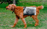
Figure 1. Area of test radiographs [click to enlarge]
Measuring
The dog should be anaesthetised and the grid properly positioned. To accurately measure the part to be radiographed, place the dog in lateral recumbency and measure its thickness at the level of the 12th rib with calipers. If the measurement is an intermediate value (such as 13.4cm) record the next highest whole number.
What mA and exposure time?
Because a grid will be used during these test exposures, 10-20mAs should be selected. Do this by setting the machine for a high mA and an exposure time (in seconds) that will provide the desired mAs. Table 1 lists some useable mAs values for X-ray machines that allow an output of 300mA.
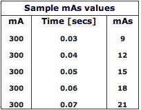
Table 1: Calculating mAs values
If your X-ray machine is a condenser-discharge or high-frequency unit, select the mAs value directly off the control panel.
Initial kVp setting
To determine the kVp for the first of the three test exposures I have modified Santes Rule and suggest that you calculate the kVp using the following formula.
(measured thickness in centimetres x 2) + 40 = initial kVp
For example, if your dog measures 14cm thickness at the 12th rib, the initial kVp should be 68. If your X-ray machine cannot generate the exact kVp required, select the nearest available setting to the one calculated.
Test radiographs
Make the first exposure using the settings calculated from the above steps. Then, make two additional exposures, one using 50% more mAs and the other 50 mAs less, than the first exposure.
Processing
Process all three images simultaneously. For manual processing, use fresh chemistry at 18-22°C. Optimal developing time is four minutes.
Evaluate
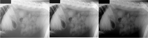
Examine the films after processing (Figure 2) to determine which if any contains an optimal image of the abdomen.
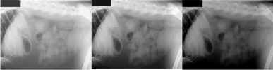
Figure 2: Test radiographs of selected area [click to enlarge].
If none of the films contains an optimal image of the abdomen, you will have to decide whether the radiographs are underexposed (too light) or overexposed (too dark).
Underexposure
To correct for underexposure, add 10 per cent to the kVp setting used for the first test exposure or double the exposure time used to produce this radiograph and use the new values to make the first of three new test exposures using the method described under Test radiographs. Evaluate each radiograph in this second series for an optimal image of the abdomen.
Overexposure
To correct for overexposure, subtract 10 per cent from the kVp setting used for the first test exposure or halve the exposure time used to produce this radiograph and use the new values to make the first of three new test exposures using the method described under Test radiographs. Evaluate each radiograph in this second series for an optimal image of the abdomen.
You may have to repeat this process once more to finetune your exposures, but persevere until you produce one good image of the abdomen. This is your successful test exposure of the abdomen. Record the thickness [at the 12th rib] and kVp and mAs [or mA and time] values in the appropriate space in table 3.
Next, we will modify the process that you used for the abdomen to obtain optimal views of the spine and thorax.
Because the skeleton is optimally viewed using a low kVp technique, select a kVp setting that is 15 kVp less that the one used for your successful abdominal exposure. To compensate for underexposure, treble the mAs used for the successful abdominal exposure. This adjustment will give you the starting trial exposures for the vertebral column. Take two more trial exposures, on using 50% more mAs, the other with 50% less mAs than used for the first exposure of the vertebral column.
For the thorax we prefer to use a high kVp technique, so select a kVp setting that is 15 kVp more that that used for your successful abdominal exposure. To compensate for overexposure, set a starting mAs value that is 1/3rd of that used for the abdomen. Take two additional thoracic exposures, varying the mAs by +/- 50% respectively.
When measuring the patient for the spine and thorax exposures, use tissue thickness at the 12th rib, as was done for the abdominal exposure.
Now, after making three test exposures of the spine and of the thorax based using these new settings, review your results. You may have to make some additional mAs adjustments until you have produce one good image of the thorax and of the abdomen. Record the exposure values used for each successful exposure in table 3.
Figure 3: Successful radiographs selected as the basis for your technique charts [click to enlarge].
Record
After you decide which exposure contains the most successful radiographic image of each body part, record the relevant kVp and mAs in the appropriate place in Table 3.
At this stage your exposure table should look like table 2:
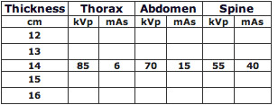
Table 2: Initial technique chart structure
Table 3 will become YOUR kVp-variable chart. As you work through the next few steps and complete the chart, remember that kVp will be the only value that changes in response to tissue depth. The mAs setting for each body part -- thorax, abdomen and spine -- will remain the same as the setting that produced its successful test exposure. Use Table 4 to record all the other details relating to these exposures.
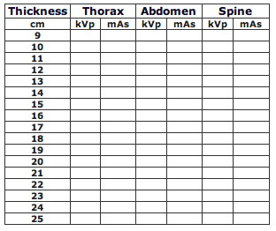
Table 3: Your technique chart
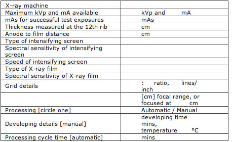
Table 4: Successful Test Exposure Specifications
Congratulations. You have completed the important task of data acquisition for your new technique chart. In the next section you will extrapolate your data and create a chart.
<< Previous chapter "Introduction" Next chapter "Creating" >>
|