|
Welcome to a VIA Online Learning Tutorial: This site has been developed to provide learning materials to enable you to create X-ray exposure charts.
Select Chapter:
1. INTRODUCTION
2. STARTING
3. CREATING [print this page]

Constructing your reference chart
The next step is to return to your reference chart (Table 2) and extrapolate the remaining kVp values for the thorax, abdomen and spine from your successful test exposures.
1) From the row displaying the successful test exposures for the thorax, abdomen and spine, work down the kVp columns until you reach the row for thicknesses of 25cm, adding 2kVp for each centimetre increase in tissue depth for exposures less than 80kVp; 3kVp for each centimetre increase in tissue depth for exposures between 80kVp and 100kVp; and 4kVp for each centimetre increase in tissue depth for exposures greater than 100kVp.
2) From the row displaying the successful test exposures for the thorax, abdomen and spine, work up each of the kVp columns until you reach the row for thicknesses of 9cm, subtracting 2kVp for each centimetre decrease in tissue depth for exposures less than 80kVp and 3kVp for each centimetre decrease in tissue depth for exposures between 80kVp and 100kVp (Table 4).
To check your work so far, compare your reference chart to the effect these calculations have on the example chart:
Table 4.
Fill in
To complete your reference chart, fill in the columns that refer to the settings for mA and seconds for the thorax, abdomen and spine. Against each tissue depth, simply enter the same mA and seconds you used to produce the successful test exposure of the relevant body part.
The completed example reference chart looks like this:
Table 5.
Although this type of chart — which allows the X-ray machine operator to adjust X-ray penetration in proportion to patient thickness — would be the ideal radiographic ready reckoner for your exposure factors, it cannot be used with a machine that has linked kVp and mA settings, so you will need to take the additional step of converting your reference chart to a mAs-variable chart.
Converting your reference chart to a mAs-variable chart
To construct your own mAs-variable chart in Table 6, you will need to refer to the values you calculated when you built your reference chart in Table 2 shown here.
Table 6: mAs-variable Chart
By following an established formula it is possible to substitute changes in mAs for changes in kVp and maintain equivalent radiographic density. This formula indicates, for example, that for kVp settings between 51 and 60, if we halve the mAs, adding 10kVp will maintain comparable radiographic density. Conversely, if we double the mAs, subtracting 10kVp will produce a radiograph of equivalent density. Expressed differently, for a kVp settings between 51 and 60, we can double or halve the mAs to compensate for decreases or increases of 10kVp respectively.
The principle of halving or doubling the mAs to reciprocate for changes in kVp is not linear across the whole range of available kVp - a sliding scale (Table 7) applies.
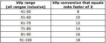
Table 7: kVp-mAs Radiographic Density Equivalents
Substitute NEW kVp and mAs settings
In this step you will convert the thoracic exposures in your reference chart (Table 2) to make them mAs variable. To make this conversion while maintaining the optimal radiographic density you have selected for your exposures, you will need to apply the principle of radiographic density equivalents outlined in Table 7. For example, the values for the thorax in example reference chart shown here, reproduced below:
...will become an mAs-variable chart that begins by looking like this:
[Table Text: 1. The mAs has been halved at a depth of 9cm to compensate for changing the kVp setting from 50 to 60 (adding 10kVp; Table 7) 2. The mAs has been doubled at a depth of 19cm to compensate for changing the kVp setting from 70 to 60 (subtracting 10kVp; Table 7) 3. The mAs has been doubled again at a depth of 25cm because at 61-70kVp this is the radiographic density equivalent of adding 12kVp (Table 7)].
By following this example you should be able to use the values from your own reference chart (Table 1) shown here, to complete the corresponding information in your mAs-variable chart (Table 3) on shown here.
Interpolate
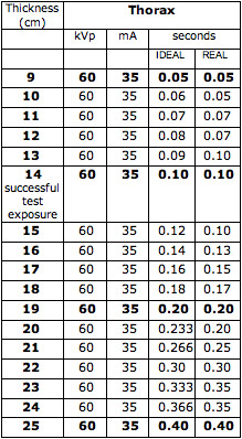
By substituting new mAs values (in this instance, by altering the exposure times) at appropriate intervals, a scaffold has been constructed that will enable the creation of a complete mAs- variable chart. The next step is to fill the scaffold with theoretical ideal time settings that correspond to the sequential steps of added tissue thickness. In the example, the values for the thorax will become:
Now return to the framework for your own mAs-variable chart (Table 6) and interpolate your own theoretical ideal exposure times.
Some of these values will appear to be quite odd because they won't correspond with the available exposure settings on your X-ray machine. Don't worry, you are about to learn how to substitute useable exposure settings. Begin by making a list of the available exposure settings on your X-ray machine, then choose the ones that most closely match the calculated "ideal" times on your mAs-variable chart (Table 6). If for example, the machine that produced the example chart was capable of the following exposure times (in seconds): 0.03, 0.05, 0.07, 0.10, 0.13, 0.15, 0.17, 0.20, 0.25, 0.30, 0.35 and 0.40, the completed example mAs-variable chart would look like this:
All X-ray machines have exposure settings greater than 0.40 seconds but they are wildly impractical and should be excluded from radiograph exposure charts.
To complete the substitution, erase all the theoretical ideal time values. By comparing your mAs-variable chart with your reference chart, you should be able to see immediately that the kVp-variable model has exceptional finetuning where it matters — in the kVp area. The mAs-variable model has coarser exposure control, which is determined by the number of available exposure time settings. If exposure timers had infinite variability, one could theoretically construct an mAs-variable chart with similar fine control to a kVp-variable chart.
Modifying factors
Under certain circumstances, the exposure time will need to be increased or decreased from the value indicated by a standard mAs-variable chart. For example, increased opacity due to fluid will cause a radiograph at a standard exposure to be underexposed if the patient has ascites or pleural effusion. Table 8 presents a useful guide to common variations.
Table 8: Modifying Factors for mAs-variable Charts
Test
Your mAs-variable chart needs to be tested on a variety of animals. Record the patient thickness and exposure factors for every radiograph you take. Always check the quality of your processed films and document under- or overexposures. Be prepared to modify your chart if consistent exposure problems become apparent after using it on several subjects.
Chart failure
If your mAs-variable chart is unreliable, perhaps the reason may be one of the factors listed in Table 9. If the problem persists after you have checked each of these possibilities, go back to your test animal and repeat the original exposures to determine whether your chart is based on appropriate test exposure factors.
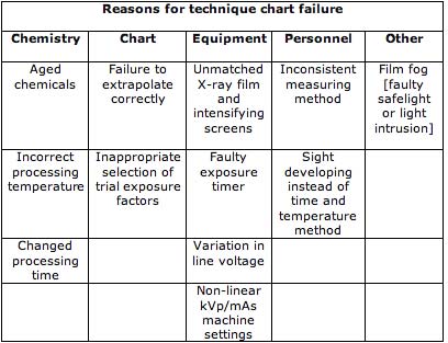
Table 9: Reasons for mAs-variable Chart Failure
Additional charts
After you have successfully completed your first chart, you are ready to make additional charts to cover the range of cases you see regularly, including:
• cats
• birds
• small exotic species, and
• small dogs that don't require a grid.
Special interest charts include those for the hips and elbows of large dogs, which are helpful in practices that regularly radiograph these joints for certification schemes.
|